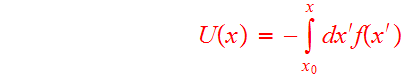
In a one-dimensional system it is always possible to define a potential energy corresponding to any given f(x); let
(1)
where ![]() is an arbitrary position at which
is an arbitrary position at which ![]() .
Different choices of
.
Different choices of ![]() produce potential energies differing by an additive constant; this
constant has no influence on the dynamics of the system.
produce potential energies differing by an additive constant; this
constant has no influence on the dynamics of the system.
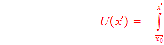
In a space of ![]() dimensions the analogous path integral,
dimensions the analogous path integral,
(2) 
![]()
may depend on the exact route taken from point ![]() to
to ![]() ;
if it does, a unique potential energy cannot be defined. One condition
for this integral to be path-independent is that the integral of the
force f(x) around all closed paths vanishes. An equivalent condition is
that there is some function U(x) such that
;
if it does, a unique potential energy cannot be defined. One condition
for this integral to be path-independent is that the integral of the
force f(x) around all closed paths vanishes. An equivalent condition is
that there is some function U(x) such that
(3) ![]()
![]()
Force fields obeying these conditions are conservative. The
gravitational field of a stationary point mass is the simplest example
of a conservative field; the energy released in moving from ![]() to
to ![]() with
with ![]() is exactly equal to that consumed in moving back from
is exactly equal to that consumed in moving back from ![]() to
to ![]() .
.
In simulation projects it's natural to work with the
path integral of the acceleration rather than the force; this integral
is the potential energy per unit mass or gravitational potential, ![]() ,
and the potential energy of a test mass m is just
,
and the potential energy of a test mass m is just ![]() .
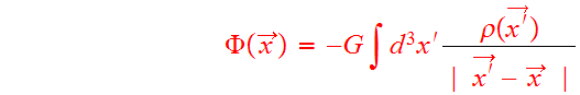
For an arbitrary mass density
.
For an arbitrary mass density ![]() ,
the potential is
,
the potential is
(4) 
![]()
where ![]() is the gravitational constant and the integral is taken over all space.
Poisson's equation provides another way to express the relationship
between density and potential:
is the gravitational constant and the integral is taken over all space.
Poisson's equation provides another way to express the relationship
between density and potential:
(5) ![]()
![]()
![]()
Note that this relationship is linear; if ![]() generates
generates ![]() and
and ![]() generates
generates ![]() then
then ![]()
![]() generates
generates ![]() .
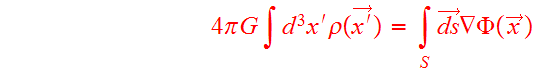
Gauss's theorem relates the mass within some volume V to the gradient
of the field on its surface:
.
Gauss's theorem relates the mass within some volume V to the gradient
of the field on its surface:
(6) 
![]()
where the infinitesimal vector ![]() is an element of surface area with an outward-pointing normal vector.
is an element of surface area with an outward-pointing normal vector.
Consider a spherical shell of mass ![]() :
:
(a) the acceleration inside the shell vanishes
(b) and the acceleration outside the shell is
![]() .
.
From these results, it follows that the potential of an arbitrary spherical mass distribution is
(7) 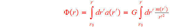
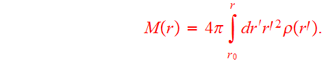
where the enclosed mass is
(8) 
A point of mass ![]() :
:
(9) ![]()
This is known as a Keplerian potential since orbits in this
potential obey Kepler's three laws. If G=1 is set, the velocity of a circular orbit at
radius ![]() is
is ![]()
A uniform sphere of mass ![]() and radius
and radius ![]() :
:
(10a) ![]()
![]()
(10b) ![]()
![]()
where ![]()
![]() is the mass density. Outside the sphere the potential is Keplerian,
while inside it has the form of a parabola; both the potential and its
derivative are continuous at the surface of the sphere.
is the mass density. Outside the sphere the potential is Keplerian,
while inside it has the form of a parabola; both the potential and its
derivative are continuous at the surface of the sphere.
Galactic potential is the collective self-consisten field of
all stars within the galaxy. It is determined by the distribution
function ![]() which accounts for the mechanical state of the galaxy.
which accounts for the mechanical state of the galaxy.
Sun is located in our Milky Way which has ![]() visible stars and about
visible stars and about ![]() solar masses of gas
solar masses of gas ![]() with
with ![]() .
In comparison,
.
In comparison, ![]() .
Gas has little effect on main features of galactic dynamics.
.
Gas has little effect on main features of galactic dynamics.
Most of the stars in the galaxy travel on nearly circular
orbits in a thin disk whose radius is of the order of ![]()
![]() and thickness of the order of
and thickness of the order of ![]()
![]() with
with ![]() .
Typical circular speed of stars is of the order of
.
Typical circular speed of stars is of the order of ![]()
![]() and the time required to complete a galactic orbit at
and the time required to complete a galactic orbit at ![]() is about
is about ![]() .
The dispersion in velocities is about
.
The dispersion in velocities is about ![]() .
Age of the galaxy
.
Age of the galaxy ![]() .
Typical disk star (like our Sun) has completed over 30 revolutions.
Galaxy is in steady state. Why and how is explained by the steady state
solution of the distribution function
.
Typical disk star (like our Sun) has completed over 30 revolutions.
Galaxy is in steady state. Why and how is explained by the steady state
solution of the distribution function ![]() from the collisionless Boltzmann equation.
from the collisionless Boltzmann equation.
Consider first a practical choice on units for galaxy
collisions: ![]() The
gravitational constant is
The
gravitational constant is ![]() in cgs units. Typical galaxy size is measured in tens of kiloparsecs,
large scale structure of the universe is measured in Megaparsecs. Let
us determine the value of
in cgs units. Typical galaxy size is measured in tens of kiloparsecs,
large scale structure of the universe is measured in Megaparsecs. Let
us determine the value of ![]() in the new galactic units:
in the new galactic units:
(11) ![]()
![]()
![]()
This value of ![]() is an inconvenient value for
is an inconvenient value for ![]() to carry in simulations. Let us try galactic units which set
to carry in simulations. Let us try galactic units which set ![]() .
One possible illustration is
.
One possible illustration is ![]() In these units
In these units
(12) ![]()
![]()
![]()
In these units we can use ![]() in the simulations. With this choice two units are arbitrary, the third
unit is fixed. There is great flexibility to interpret simulation
results in physical units at the very end of the runs with
dimensionless numbers.
in the simulations. With this choice two units are arbitrary, the third
unit is fixed. There is great flexibility to interpret simulation
results in physical units at the very end of the runs with
dimensionless numbers.
![]()
![]() astronomy units
astronomy units
![]() Kepler orbits.
Kepler orbits.
![]()
![]() Kepler orbits (1
earth year)
Kepler orbits (1
earth year) ![]() one Saturn year
one Saturn year