Lecture 8/9: Galaxy collisions with spherical potential
Physics 141/241
Orbits in Spherical Potentials
Consider the motion of a star in a spherically-symmetric potential,
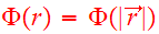 .
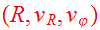
The orbit of the star remains in a plane perpendicular to the angular momentum
vector, and it's natural to adopt a polar coordinate system; call the
coordinates
.
The orbit of the star remains in a plane perpendicular to the angular momentum
vector, and it's natural to adopt a polar coordinate system; call the
coordinates
 and
and
 .
The system has
.
The system has
 degrees of freedom, so the phase space has
 dimensions.
The equations of motion can be derived by starting with the Lagrangian
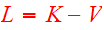 ,
,
(1)
 ,
,
where
 and
and
 .
In what follows, we will use a choice of unit mass and
.
In what follows, we will use a choice of unit mass and
 will not show in the equations:
(2)  .
.
Differentiating with respect to
 and
and
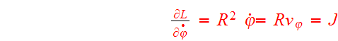
 yields the momenta conjugate to
 and
and
 ,
,
(3)
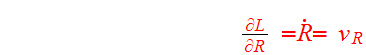 ,
,
(4)
 ,
,
where
 and
and
 are velocities in the radial and azimuthal directions. The Hamiltonian
(energy) may now be expressed as a function of the coordinates and conjugate
momenta:
are velocities in the radial and azimuthal directions. The Hamiltonian
(energy) may now be expressed as a function of the coordinates and conjugate
momenta:
(5)
 .
.
The equations of motions are
(6)
 ,
,
(7)
 ,
,
(8)
 ,
,
(9)
 .
.
Here
 because the conjugate coordinate phi does not appear in
 ;
;
 is
called a cyclic coordinate.
is
called a cyclic coordinate.
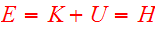
The system has two integrals of motion. One, of course, is the total energy
 ,
numerically equal to the value of
,
numerically equal to the value of
 .
The other is the angular momentum
.
The other is the angular momentum
 .
These quantities are given by
.
These quantities are given by
(10)
 ,
,
(11)
 .
.
Each of these integrals of motion defines a hypersurface in phase space, and
the orbit must remain in the intersection of these hypersurfaces. This can be
visualized by ignoring the
 coordinate and drawing surfaces of constant
 and J in the three-dimensional space
 .
Surfaces of constant
.
Surfaces of constant
 are figures of revolution about the
 axis, while surfaces of constant
 are hyperbolas in the
 plane. The intersection of these surfaces is a closed curve, and an orbiting
star travels around this curve.
plane. The intersection of these surfaces is a closed curve, and an orbiting
star travels around this curve.
For an orbit of a given
 ,
the system may be reduced to one degree of freedom by defining the effective
potential,
,
the system may be reduced to one degree of freedom by defining the effective
potential,
(12)
 ;
;
the corresponding equations of motion are then just
(13)

 ,
,
(14)

 .
.
Because
 diverges as
 ,
the star is energetically prohibited from coming too close to the origin, and
shuttles back and forth between turning points
,
the star is energetically prohibited from coming too close to the origin, and
shuttles back and forth between turning points
 and
and
 .
.
In addition to its periodic radial motion described by
 ,
a star also executes a periodic azimuthal motion as it orbits the center of
the potential. If the radial and azimuthal periods are incommensurate, as is
usually the case, the resulting orbit never returns to its starting point in
phase space; in coordinate space such an orbit is a rosette. The Keplerian
potential is a very special case in which the radial and azimuthal periods of
all bound orbits are equal. The only other potential in which all orbits are
closed is the harmonic potential generated by a uniform sphere; here the
radial period is half the azimuthal one and all bound orbits are ellipses
centered on the bottom of the potential well. Thus in the Keplerian case all
stars advance in azimuth by
,
a star also executes a periodic azimuthal motion as it orbits the center of
the potential. If the radial and azimuthal periods are incommensurate, as is
usually the case, the resulting orbit never returns to its starting point in
phase space; in coordinate space such an orbit is a rosette. The Keplerian
potential is a very special case in which the radial and azimuthal periods of
all bound orbits are equal. The only other potential in which all orbits are
closed is the harmonic potential generated by a uniform sphere; here the
radial period is half the azimuthal one and all bound orbits are ellipses
centered on the bottom of the potential well. Thus in the Keplerian case all
stars advance in azimuth by
 between successive pericenters, while in the harmonic case they advance by
 .
Galaxies typically have mass distributions intermediate between these extreme
cases, so most orbits in spherical galaxies are rosettes advancing by
.
Galaxies typically have mass distributions intermediate between these extreme
cases, so most orbits in spherical galaxies are rosettes advancing by
 between pericenters.
N-body Equations of Motion
Any system in which stellar collisions are rare may be idealized as a
collection of
 point-sized bodies, each with mass
 ,
position
,
position
 ,
and velocity
,
and velocity
 .
The hamiltonian for such a system is
.
The hamiltonian for such a system is
(15)
 ,
,
where
 depends on all body positions and velocities, the first sum runs over all
 bodies, the second runs over all pairs of bodies (twice, hence the factor of
 ),
and
),
and
 is the gravitational constant. Then the equations of motion are
(16)
 ,
,
(17)
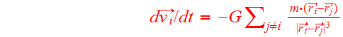 ,
,
where the sum runs over all bodies except body
 .
.
The famous Aarseth code in Fortran (Aarseth Fortran
code) calculates the general motion of the N-body system in computer
simulations.
N-body systems obey several basic conservation laws. A symmetry of the
Hamiltonian is a transformation which leaves the physical system unchanged.
For example, translation in time,
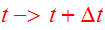 ,
is a symmetry of Eq. 15 because
,
is a symmetry of Eq. 15 because
 is not an explicit function of time; consequently the total system energy
 is conserved. Likewise, symmetry with respect to translation in space
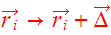 ,
implies conservation of total linear momentum, and symmetry with respect to
rotation gives rise to conservation of total angular momentum.
,
implies conservation of total linear momentum, and symmetry with respect to
rotation gives rise to conservation of total angular momentum.
Virial Parameters
Another general result shown by manipulating Eqs. 16,17 is the scalar virial
theorem which states that for a system in equilibrium,
(18)

where
 and
and
 are the total kinetic and potential energy, respectively, and the
angle-brackets indicate time-averages. Since
are the total kinetic and potential energy, respectively, and the
angle-brackets indicate time-averages. Since
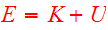 ,
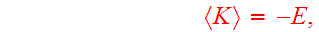
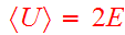
the time-averaged kinetic and potential energies are related to the conserved
total energy by
,
the time-averaged kinetic and potential energies are related to the conserved
total energy by
(19)
 .
.
The total mass
 and total energy
 of an N-body system thus define characteristic velocity and length scales
(20)
 ,
,
(21)
 .
.
These are sometimes known as the virial velocity and radius, respectively.
The quantity
 is an estimate of the time a typical star takes to cross the system. This
timescale may be expressed in several different ways; for example, in terms of
the total mass
is an estimate of the time a typical star takes to cross the system. This
timescale may be expressed in several different ways; for example, in terms of
the total mass
 and energy
 ,
it is
,
it is
(22)
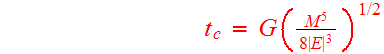 .
.
Note that
 and
and
 are conserved, so
 is a constant even for systems which are far from dynamical equilibrium. In
such cases
is a constant even for systems which are far from dynamical equilibrium. In
such cases
 approximates the time-scale over which the system evolves toward equilibrium.
Another expression for
 follows from the substitution
 valid for systems near equilibrium:
(23)
 .
.
Here the quantity
 ,
which has units of density, appears. In systems with galaxy-like density
profiles, the virial radius is approximately proportional to the half-mass
radius:
,
which has units of density, appears. In systems with galaxy-like density
profiles, the virial radius is approximately proportional to the half-mass
radius:
 .
Using this relationship, it follows that
.
Using this relationship, it follows that
(23)
 ,
,
where
 is the mean density within
 .
Since the crossing time is just supposed to indicate a typical time-scale for
orbital motion, it is usual to drop the numerical constant, and define
.
Since the crossing time is just supposed to indicate a typical time-scale for
orbital motion, it is usual to drop the numerical constant, and define
(24)
 .
.