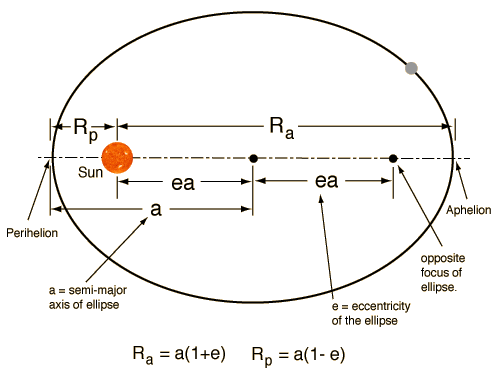
Each plane has an elliptic orbit, with the Sun in a focus point:
The total energy of the planet of mass ![]() is given by
is given by
(1) ![]()
where ![]() is the mass of the Sun and
is the mass of the Sun and ![]() is the angular momentum of the orbit (see Lecture 4).
Setting
is the angular momentum of the orbit (see Lecture 4).
Setting ![]() at perihelion, the following relation holds for the minimal planet-Sun
distance
at perihelion, the following relation holds for the minimal planet-Sun
distance
(2) ![]()
which can be expressed in terms of the geometry of the orbit
(3) ![]()
![]() .
.
This allows us to express the azimuthal velocity at perihelion in terms of the geometry and masses using the Astrophysical tables.
We want to open a new visual editor in DX and put on the canvas the modules with connections which will look like this. We will work with the data file sphere.data which has 51 frames with 2,000 mass points for each frame. The data file was generated with the Aarseth code and describes the gravitaional collapse of a spherical mass point distribution uniformly and randomly filling the sphere of unit radius with zero starting velocities. We have to bring in the data into DX which is controlled by sphere.general which communicates the arrangement of the data to DX. This requires to reprogram module Import as shown in the figure. We also have to reprogram the Sequencer module. The other modules do not require any reprogramming for a start. This allows us to run the animation but the visual display will show large glyphs. This can be modified later by reprogramming the Glyph module. This setup can be used with easy adaptation for any animation of data files generated by N-body simulations.
We have to load into the Visual Program Editor the MPEGmac.net macro module, put it on the canvas and make the connections with the Image and Sequencer modules. The canvas will look like this. No further reprogramming of the modules is required. Running the visual program will run the animation now and generate a YUV file for each frame with another file containing the size information in pixels. After a full run, 51 YUV images are created which can be encoded into the mpeg movie using mpeg_encode as described in Lab Session 2 here.